Create Extended Funnel Plots — extfunnel2 • extfunnel2

Inspired by the archived extfunnel package by Langan et al. The function creates an extended funnel plot with shaded contours that show the impact of a new study with a certain effect estimate and standard error (or sample size) on the conclusions of an updated meta-analysis. Uses ggplot2 instead of base R, allows specification of the meta-analytic model via the metafor package as well as simulation using sample size per group.

Usage

extfunnel2(
  yi,
  sei,
  sd = NULL,
  n = NULL,
  swe,
  method = "REML",
  test = "z",
  contour_points = 50,
  x_lim,
  y_lim,
  x_lab = "Effect size",
  y_lab = "Standard error",
  x_ticks = NULL,
  y_ticks = NULL,
  legend_pos = "right",
  legend_just = NULL,
  exp = FALSE
)

Arguments

yi: A numeric vector with effect estimates for each study. Odds/ risk ratios should be log-transformed.
sei: A numeric vector with standard errors for each study. Must be specified. If 'sd' and 'n' are not specified the y-axis will correspond to the standard error.
sd: A single numeric value corresponding to the assumed standard deviation per group of a future study. If 'sd' and 'n' are specified the y-axis will correspond to the sample size per group. Only works for mean differences.
n: A numeric vector of the average sample size per group for each study. Only needed when 'sd' is specified.
swe: A single numeric value corresponding to the smallest worthwhile effect. Odds/ risk ratios should be log-transformed.
method: A character string indicating which method should be used to estimate tau. Default is "REML". See rma of the metafor package for more options.
test: A character string indicating which method should be use to calculate confidence intervals. Default is "z". See rma of the metafor package for more options.
contour_points: A numeric value indicating the number of contour points to be used for simulation. Default is 50. For high quality contours 500 is recommended. This takes a long time as 250.000 (500x500) meta-analyses will run (one contour point equates to one meta-analysis).
x_lim: A numeric vector with two values indicating the lower and upper limits of the simulated effect estimates (corresponds to x-axis limits). Odds/ risk ratios should be log-transformed.
y_lim: A numeric vector with two values indicating the lower and upper limits of the simulated standard errors (corresponds to y-axis limits). If 'sd' and 'n' are provided 'y_lim' corresponds to the lower and upper limits of the sample size per group.
x_lab: A character string indicating the x-axis label for the plot. Default is "Effect size".
y_lab: A character string indicating the y-axis label for the plot. Default is "Standard error".
x_ticks: A numeric vector indicating the tick marks for the x-axis. Default is NULL. Odds/ risk ratios should be log-transformed.
y_ticks: A numeric vector indicating the tick marks for the y-axis. Default is NULL.
legend_pos: A character string indicating the position of the legend in the plot. Default is "right". Can be "top", "right", "bottom", or "left".
legend_just: A character string indicating the legend justification in relation to the 'legend_pos' argument. Default is NULL. I.e. if 'legend_pos' is "right" and 'legend_just' top, the legend will appear at the top right corner of the plot.
exp: A logical value indicating whether the x-axis should be on a logarithmic scale (in case odds/ risk ratios are provided). Default is FALSE.

Value

An extended funnel plot (ggplot2 object) with shaded contours that show the impact of a new study with a certain effect estimate and standard error (or sample size) on the conclusions of an updated meta-analysis.

Acknowledgments

Langan, D., Sutton, A. J., Higgins, J. P. T. & Gregory, W. (2013). extfunnel. R package version 1.3. https://cran.r-project.org/package=extfunnel
Langan, D., Higgins, J. P. T., Gregory, W., & Sutton, A. J. (2012). Graphical augmentations to the funnel plot assess the impact of additional evidence on a meta-analysis. Journal of Clinical Epidemiology, 65(5), 511–519. https://doi.org/10.1016/j.jclinepi.2011.10.009
Ferreira, M. L., Herbert, R. D., Crowther, M. J., Verhagen, A., & Sutton, A. J. (2012). When is a further clinical trial justified? BMJ, 345, e5913. https://doi.org/10.1136/bmj.e5913
Wickham, H. (2016). ggplot2: Elegant Graphics for Data Analysis. Springer-Verlag New York. https://ggplot2.tidyverse.org
Viechtbauer, W. (2010). Conducting meta-analyses in R with the metafor package. Journal of Statistical Software, 36(3), 1-48. https://doi.org/10.18637/jss.v036.i03

Author

Florian Teichert teichert.florian@gmail.com
ORCID 0000-0003-2211-797

Examples

# Load package once installed
library(extfunnel2)

# Reproducing the extended funnel plot from Ferreira et al. 2012
# Random effects meta-analysis (effect of exercise on chronic low back pain)
data <- data.frame(yi = c(-10.0, -16.3, -27.0, -14.0, -15.1, -2.1, -19.0, -8.7),
                   sei = c(3.4, 5.8, 3.4, 5.3, 2.9, 1.1, 7.2, 4.2),
                   ni = c(174.0, 35.0, 25.0, 30.5, 13.5, 34.0, 15.0, 86.0))

# Create extended funnel plot
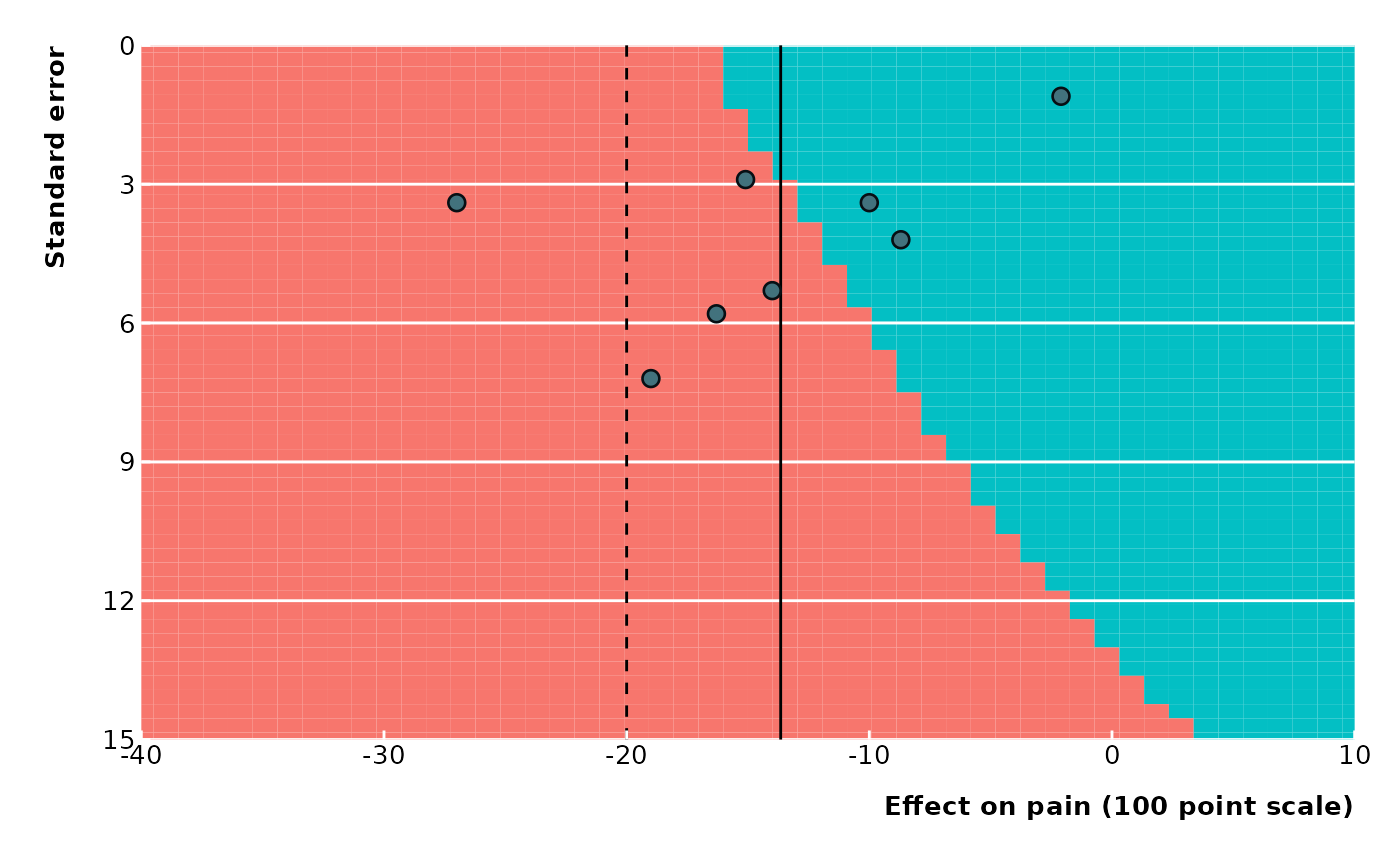
# Standard error on y-axis
extfunnel2(data$yi, data$sei,
           swe = -20,
           method = "DL",
           contour_points = 50,
           x_lim = c(-40, 10), y_lim = c(0, 15),
           x_ticks = seq(from = -40, to = 10, by = 10),
           y_ticks = seq(from = 0, to = 15, by = 3),
           x_lab = "Effect on pain (100 point scale)",
           legend_pos = "none"
           )


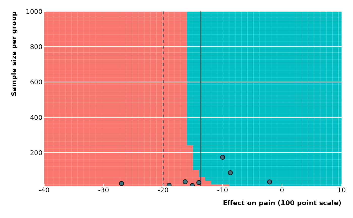
 # Sample size per group on y-axis
 # Assumptions: Equal group sizes and fixed SD
 extfunnel2(data$yi, data$sei,
            sd = 15, n = data$ni,
            swe = -20,
            method = "DL",
            contour_points = 50,
            x_lim = c(-40, 10), y_lim = c(10, 1000),
            x_ticks = seq(from = -40, to = 10, by = 10),
            y_ticks = seq(from = 0, to = 1000, by = 200),
            x_lab = "Effect on pain (100 point scale)",
            y_lab = "Sample size per group",
            legend_pos = "none"
            )


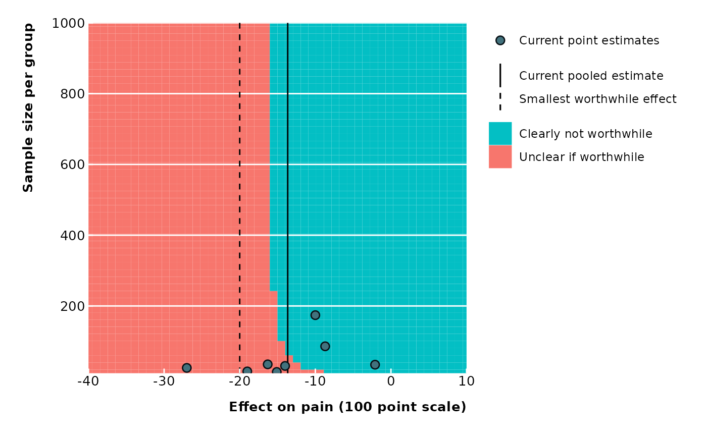
 # With legend
 extfunnel2(data$yi, data$sei,
            sd = 15, n = data$ni,
            swe = -20,
            method = "DL",
            contour_points = 50,
            x_lim = c(-40, 10), y_lim = c(10, 1000),
            x_ticks = seq(from = -40, to = 10, by = 10),
            y_ticks = seq(from = 0, to = 1000, by = 200),
            x_lab = "Effect on pain (100 point scale)",
            y_lab = "Sample size per group",
            legend_just = "top"
            )